


Next: Linear Vector Spaces in
Up: Mathematical Background
Previous: Unitary Operators
The commutator, defined in section 3.1.2, is
very important in quantum mechanics. Since a definite value of
observable A can be assigned to a system only if the system is in an
eigenstate of  ,
then we can simultaneously assign definite
values to two observables A and B only if the system is in an
eigenstate of both
and
,
then we can simultaneously assign definite
values to two observables A and B only if the system is in an
eigenstate of both
and  .
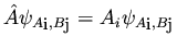
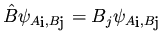
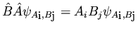
Suppose the system has a
value of Ai for observable A and Bj for observable B. The we
require
.
Suppose the system has a
value of Ai for observable A and Bj for observable B. The we
require
 |
|
|
(64) |
 |
|
|
|
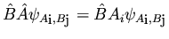
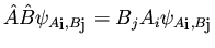
If we multiply the first equation by
and the second by
then we obtain
 |
|
|
(65) |
 |
|
|
|
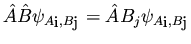
and, using the fact that
 is an eigenfunction of and ,
this becomes
is an eigenfunction of and ,
this becomes
 |
|
|
(66) |
 |
|
|
|
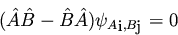
so that if we subtract the first equation from the second, we obtain
 |
(67) |
For this to hold for general eigenfunctions, we must have
 ,
or
,
or
![$[\hat{A}, \hat{B}] = 0$](/Quantum%20Mechanics/Tutorial/notes/quantum_doc/img67.png) .
That is, for two
physical quantities to be simultaneously observable, their operator
representations must commute.
.
That is, for two
physical quantities to be simultaneously observable, their operator
representations must commute.
Section 8.8 of Merzbacher [2] contains some useful
rules for evaluating commutators. They are summarized below.
![\begin{displaymath}[ {\hat A}, {\hat B} ]+ [ {\hat B}, {\hat A} ] = 0
\end{displaymath}](/Quantum%20Mechanics/Tutorial/notes/quantum_doc/img139.png) |
(68) |
![\begin{displaymath}[ {\hat A} , {\hat A} ]= 0
\end{displaymath}](/Quantum%20Mechanics/Tutorial/notes/quantum_doc/img140.png) |
(69) |
![\begin{displaymath}[ \hat{A}, \hat{B} + \hat{C} ]= [ \hat{A}, \hat{B} ]
+ [ \hat{A}, \hat{C} ]
\end{displaymath}](/Quantum%20Mechanics/Tutorial/notes/quantum_doc/img141.png) |
(70) |
![\begin{displaymath}[ \hat{A} + \hat{B}, \hat{C} ]= [ \hat{A}, \hat{C} ]
+ [ \hat{B}, \hat{C} ]
\end{displaymath}](/Quantum%20Mechanics/Tutorial/notes/quantum_doc/img142.png) |
(71) |
![\begin{displaymath}[ \hat{A}, \hat{B} \hat{C} ]= [ \hat{A}, \hat{B} ]
\hat{C} + \hat{B} [\hat{A}, \hat{C} ]
\end{displaymath}](/Quantum%20Mechanics/Tutorial/notes/quantum_doc/img143.png) |
(72) |
![\begin{displaymath}[ \hat{A} \hat{B}, \hat{C} ]= [ \hat{A}, \hat{C} ]
\hat{B} + \hat{A} [\hat{B}, \hat{C} ]
\end{displaymath}](/Quantum%20Mechanics/Tutorial/notes/quantum_doc/img144.png) |
(73) |
![\begin{displaymath}[ \hat{A}, [ \hat{B}, \hat{C} ]]
+ [\hat{C}, [ \hat{A}, \hat{B}] ] +
[ \hat{B}, [ \hat{C}, \hat{A}] ] = 0
\end{displaymath}](/Quantum%20Mechanics/Tutorial/notes/quantum_doc/img145.png) |
(74) |
If
and
are two operators which commute with their
commutator, then
![\begin{displaymath}[\hat{A}, \hat{B}^{n}]= n \hat{B}^{n-1} [\hat{A}, \hat{B}]
\end{displaymath}](/Quantum%20Mechanics/Tutorial/notes/quantum_doc/img146.png) |
(75) |
![\begin{displaymath}[\hat{A}^{n}, \hat{B}]= n \hat{A}^{n-1} [\hat{A}, \hat{B}]
\end{displaymath}](/Quantum%20Mechanics/Tutorial/notes/quantum_doc/img147.png) |
(76) |
We also have the identity (useful for coupled-cluster theory)
![\begin{displaymath}e^{\hat{A}} \hat{B} e^{-\hat{A}} = \hat{B} + [\hat{A},\hat{B}...
...{1}{3!} [ \hat{A}, [ \hat{A}, [ \hat{A}, \hat{B}] ] ] + \cdots
\end{displaymath}](/Quantum%20Mechanics/Tutorial/notes/quantum_doc/img148.png) |
(77) |
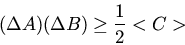
Finally, if
![$[ \hat{A}, \hat{B} ] = i \hat{C}$](/Quantum%20Mechanics/Tutorial/notes/quantum_doc/img149.png) then the uncertainties
in A and B, defined as
then the uncertainties
in A and B, defined as
 ,
obey the
relation1
,
obey the
relation1
 |
(78) |
This is the famous Heisenberg uncertainty principle. It is easy
to derive the well-known relation
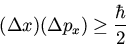 |
(79) |
from this generalized rule.
Next: Linear Vector Spaces in
Up: Mathematical Background
Previous: Unitary Operators